
Home › Mac Apps › Wolfram Mathematica

Wolfram Mathematica 15.0 (Mac)
Updated
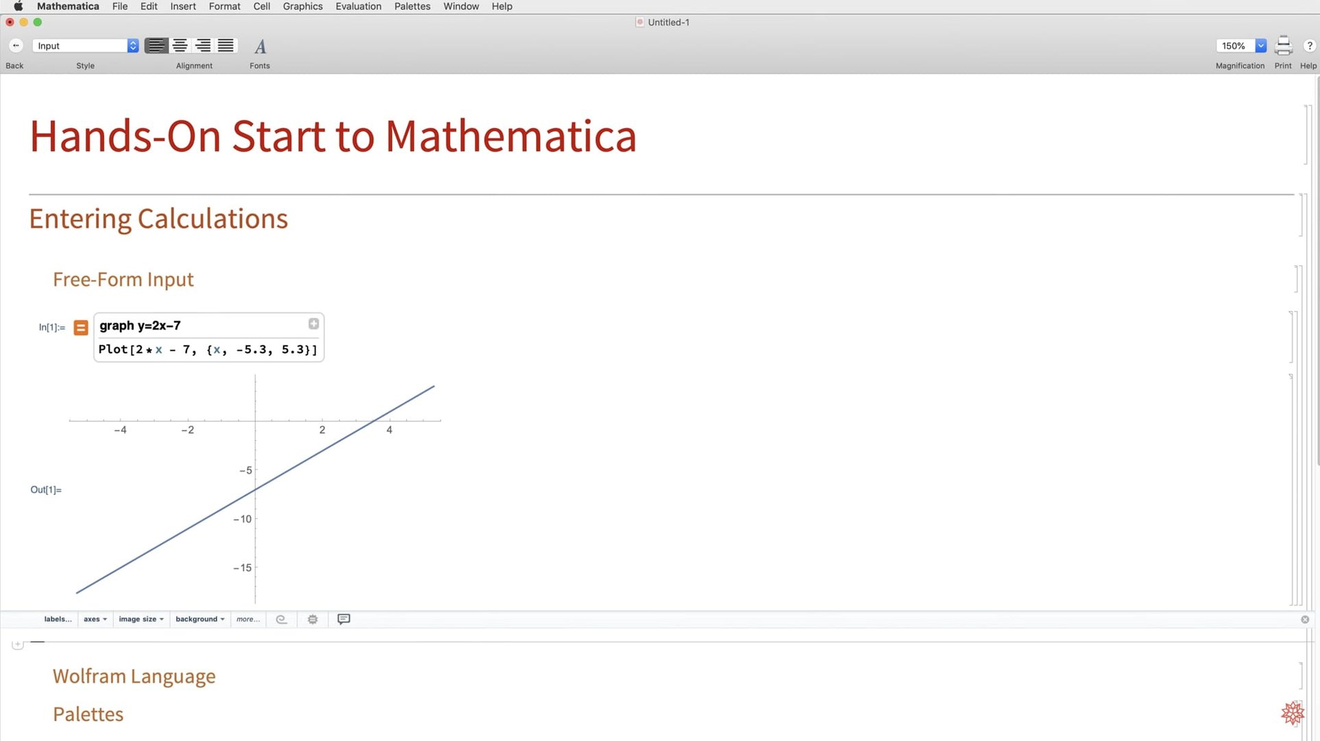
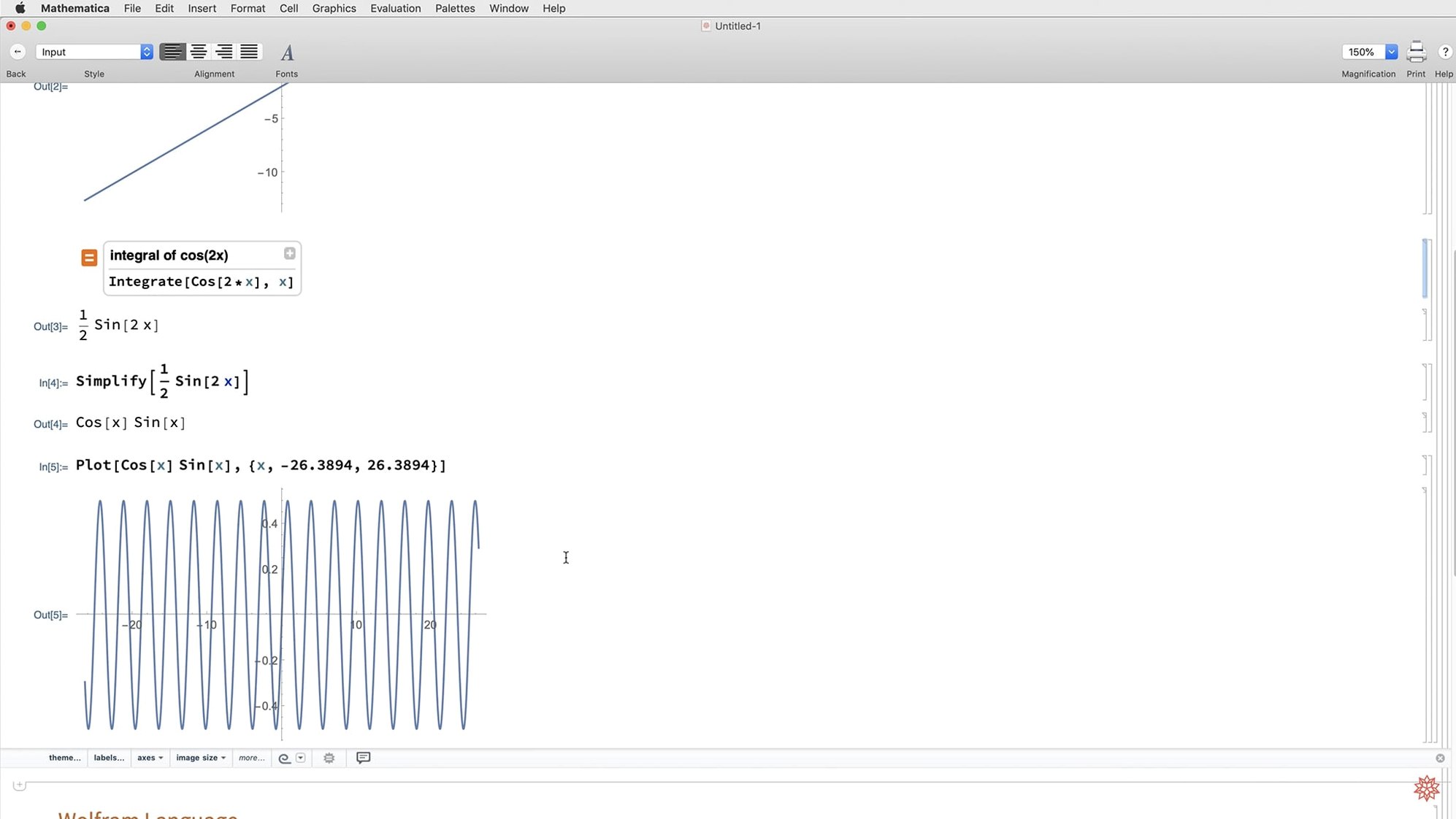
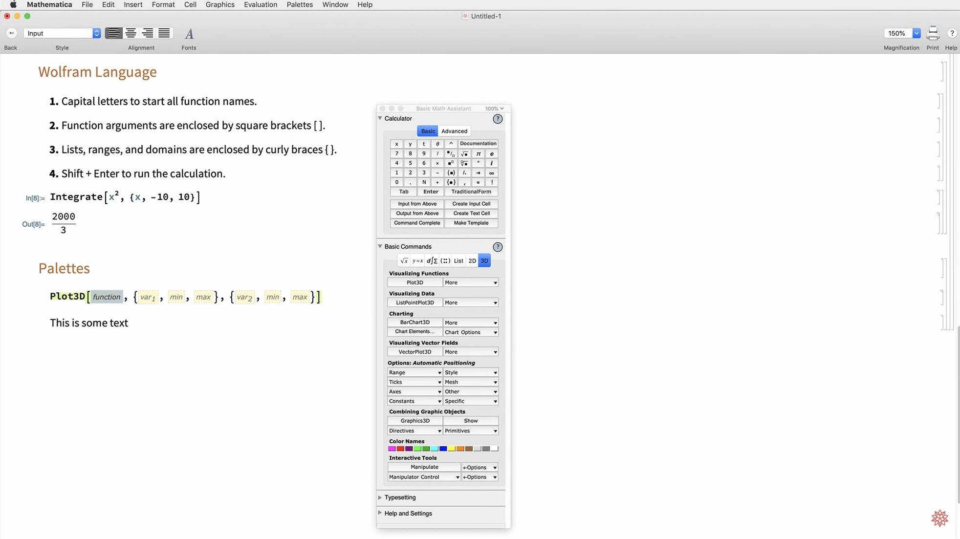
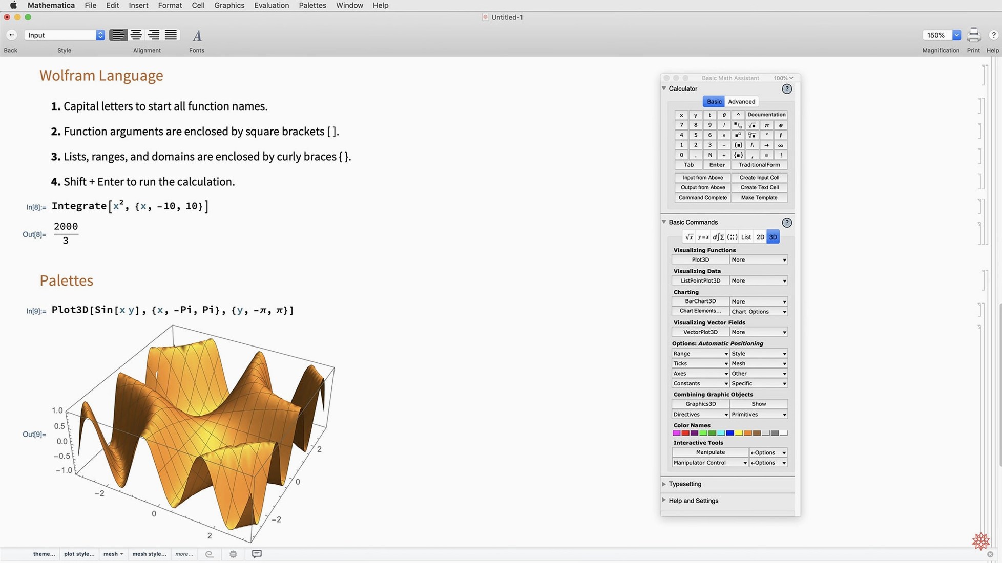
The catalogue note
Version 14.3 of Wolfram Mathematica brings a long-awaited full dark mode, with new standard colours that adapt to both dark and light environments. For someone who spends evenings staring at a notebook, that alone is a reason to look at the update. But the release also adds Hilbert transforms, Lommel functions, and fresh matrix decompositions, which means symbolic and numerical work gets a bit more coverage.
One realistic task: fitting a curve to noisy data
Say you have a set of experimental points and need a smooth fit. Start by importing the data — Mathematica handles external files easily. Then use ListFitPlot, new in 14.3, to see the points and the fitted curve in one go. The plot updates as you tweak the model, so you can compare polynomial, exponential, or custom fits without leaving the notebook. If the fit needs a surface instead of a line, the new surface plotting functions step in.
From calculation to deliverable
Once the fit looks right, you can export the result as a vector-based map or a Markdown report, both supported in this version. The notebook itself can be deployed to local or network formats, which is handy when colleagues need a readable summary. The whole flow — import, analyse, visualise, export — stays inside one tool, and the new mesh processing tools help if your data has a geometric component.
Set dark mode independently in Preferences
Before diving into a real project, a few preferences make the daily use of Mathematica more comfortable. The dark mode in version 14.3 respects system settings by default, but you can set it independently inside the Appearance tab of Preferences if you prefer a light interface during the day and dark at night. The new standard colours for plot lines and backgrounds are worth reviewing early — they default to something readable, but you might want a palette that matches your reports or your studio's branding.
Another setting I adjust first is the notebook's default style sheet. Mathematica ships with several, and switching to a print-optimised or presentation-oriented one early saves reformatting later. The interface language can be set to any of the seventeen included options; if you share a machine, each user can keep their own language without affecting system-wide settings.
Walk through acoustic data to a publication graphic
Let me walk through a session that mirrors what I do when a client brings in a set of acoustic measurements — frequency response points from a microphone test, say. I start a new notebook and type the data directly into a list, or drag a CSV file onto the notebook to import it. Natural-language input works here: typing "import measurements.csv" gets picked up without needing to remember the exact Wolfram Language syntax.
Next, I want to see what the data looks like. A quick call to ListPlot gives me a raw scatter of points. The new ListFitPlot in 14.3 is where the real work begins: I feed it the data, try a polynomial fit, then a spline. The plot updates in the same cell, so I can compare them side by side. If the fit looks off in one region, I can grab the mesh processing tools to clean up outlier points before refitting.
Once the fit is acceptable, I add labels, adjust the new standard colours for the line and the axes, and export the plot as a vector graphic — SVG or PDF — for the report. The Markdown export feature lets me embed that graphic in a text document without leaving the notebook. The whole session, from import to final export, takes one notebook and maybe half a dozen cells.
Pull data from Numbers, CSV, or clipboard paste
Mathematica does not live in isolation. On a Mac, you can pull data directly from Numbers tables, from CSV files saved by other scientific software, or from the clipboard — paste a tab-separated block from a spreadsheet, and Mathematica interprets it as a list. The new faster Python and R integration in 14.3 means you can call scripts written in those languages from inside a notebook, passing data back and forth without file exports. For a sound engineer, that is useful when your calibration script lives in Python and you want to process its output with Mathematica's symbolic tools.
Cloud access through a web browser lets you start a computation on the desktop and pick it up on a mobile device later — useful when a client asks for an adjustment while you are away from the studio. The cloud version shares the same notebooks, so nothing gets lost in translation. On macOS, the dark mode syncs with the system if you want it to, and the notebook windows behave like any other document window: Spaces, full-screen mode, and split view all work as expected. For someone who keeps a reference notebook open alongside a DAW or a text editor, that consistency matters.
Changes in this build
- Full dark mode support with new standard colours for dark and light environments.
- New matrix decompositions, Hilbert transforms, and Lommel functions.
- ListFitPlot, surface plotting, vector-based maps, and mesh processing tools.
- Geodesic computation, LLMGraph, faster Python and R integration, ColumnwiseCombine, system model validation, and Markdown export.
Before it goes on the Mac
- macOS 12 or later
- Intel or Apple Silicon
Installing it on the Mac
- Install the app following the included instructions.
- Use the included activation instructions if needed.
Notes from the control room
Sign in or open a catalogue account to leave a note.
No notes from the room yet. If you have used this build for a week, a short note helps the next person.